Beijing Multi-Site Air Quality — EDA 深潜 + Box-Cox λ 测定 + 统计基线

数据: train.csv (全量 360,954 行) · 生成时间: 2026-09-05 · 脚本: scripts/eda_compute.py → reports/eda_numbers.json → scripts/render_eda_report.py 铁律: 本报告所有数字均由 Python 实际运行产出(见文末【溯源与复现】),未手工转写。

0. 数据概况

行数 360,954 × 列数 19;时间范围 2013-03-01 00:00:00 → 2016-08-31 22:00:00 (2013-03-01 → 2016-08-31,共 42 个月)
站点 12 个: Aotizhongxin, Changping, Dingling, Dongsi, Guanyuan, Gucheng, Huairou, Nongzhanguan, Shunyi, Tiantan, Wanliu, Wanshouxigong
目标列 PM2_5_next_hour 缺失 = 0 行;数据中无 current_PM2_5 列(禁止用 PM2.5 历史做特征,泄漏红线)

1. 目标变量分布

fig1

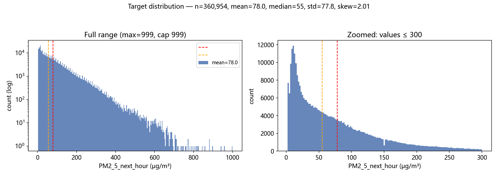
统计量	值	统计量	值
count	360,954	skew	2.01
mean	78.0	median	55
std	77.8	min / max	2 / 999 (封顶)
分位数	p1=3 / p5=6 / p25=21 / p50=55 / p75=108 / p90=179 / p95=235 / p99=354	999 封顶行数	1 行 (0.0003%)
>600 行数	197 行 (0.055%)

解读: mean(78.0) >> median(55),skew=2.01,强右偏长尾;max=999 为传感器封顶(全数据仅 1 行恰在 999,>600 共 197 行)。75% 分位才 108,但 99% 分位 354——RMSE 评分下这些尖峰事件权重极大,模型对高值事件的预测能力直接决定分数。

2. 站点差异

fig2

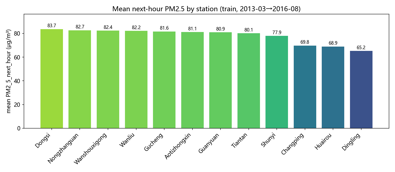
站点	均值	中位数	std	样本数	站点	均值	中位数	std	样本数
Dongsi	83.7	60	82.6	30,079	Guanyuan	80.9	59	77.6	30,199
Nongzhanguan	82.7	58	82.9	30,175	Tiantan	80.1	58	77.5	30,102
Wanshouxigong	82.4	59	81.6	30,091	Shunyi	77.9	54	78.4	29,940
Wanliu	82.2	59	79.5	30,393	Changping	69.8	46	70.1	29,992
Gucheng	81.6	59	78.5	30,166	Huairou	68.9	47	69.6	29,830
Aotizhongxin	81.1	58	79.2	29,846	Dingling	65.2	41	71.4	30,141

解读: 城区站最高 Dongsi 83.7,郊区背景站最低 Dingling 65.2,极差 ≈ 18.5 μg/m³(约 28%)。各站 std 均在 70–83,分布形状相似(右偏),主要差别在均值水平 → station 是有效的分类特征,但不足以单独解释方差。

3. 时间结构(季节性与年际)

fig3

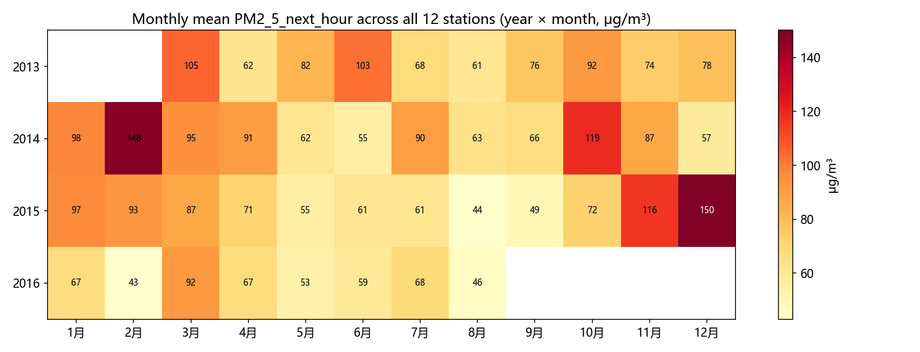
月内均值(全期、12 站合并,按自然月):

月	1	2	3	4	5	6	7	8	9	10	11	12
均值	87.1	93.5	94.7	72.7	63.0	69.1	71.8	53.4	63.9	94.3	92.0	96.0

季节规律: 采暖季(10–3月)高,暖季低;全期最低 8月 53.4,最高 12月 96.0
但年际波动巨大: 全数据最高月 2015-12月 = 150.1;最低 2016-2月 = 42.9(2016-02 反常干净;对比 2014-02 = 148.3)。
热力图 NaN 区 = 该年月不在 train 内(2013-01/02、2016-09 之后),并非缺失。

解读: 仅靠 month-of-year 类日历特征做预测,会被年际差异(如 2015-12=150 vs 2016-02=43)击穿——见 §6 基线 B2。模型应主要依赖实时污染物/气象特征承载事件信号,日历特征只做季节先验。

4. 特征与目标的相关性(Pearson,逐对剔除缺失)

特征	r	特征	r
PM10	+0.848	CO	+0.762
NO2	+0.643	SO2	+0.499
WSPM	-0.280	O3	-0.133
DEWP	+0.124	TEMP	-0.122
RAIN	-0.028	PRES	+0.022

解读: 现时污染物是下一小时 PM2.5 的最强代理——PM10 r=+0.848、CO +0.762、NO2 +0.642(同源燃烧排放,且小时级自相关强);WSPM 负相关(风扩散),O3/TEMP 弱负相关(光化学活跃期往往清洁),DEWP 弱正。这解释了 §6 中线性回归不含任何 PM2.5 历史仍能拿到低 RMSE。

5. 缺失率(按列)

列	缺失率 %	列	缺失率 %
CO	4.386	O3	2.355
NO2	2.084	SO2	1.292
PM10	0.532	wd	0.220
DEWP	0.050	PRES	0.049
TEMP	0.049	WSPM	0.048
RAIN	0.048

其余列(id/时间/station/年月日/hour/目标)缺失率为 0。解读: 缺失集中在 4 个污染物列(CO 4.4% / O3 2.4% / NO2 2.1% / SO2 1.3%),PM10 0.5%,气象列几乎无缺失 → 插补策略对 CO/O3 的稳健性比气象更重要;目标列无缺失。

6. Box-Cox λ 测定

数据前提: 目标全 >0(min=2),无需 log(y+c) 平移,可直接 Box-Cox: y(λ) = (y^λ − 1)/λ
全样本(360,954 点): scipy.stats.boxcox_normmax method='mle'(最大化变换后正态似然)→ λ = 0.1668;method='pearsonr'(最大化变换值与正态分位数相关)→ λ = 0.1905
逐站 λ(mle): 范围 0.0974(Dingling) → 0.1995(Dongsi),12 站平均 0.1639:

站点	λ	λ
Aotizhongxin	0.1573	Changping
Dingling	0.0974	Dongsi
Guanyuan	0.1652	Gucheng
Huairou	0.1493	Nongzhanguan
Shunyi	0.1655	Tiantan
Wanliu	0.1886	Wanshouxigong

与队友参考图(R fable Guerrero λ≈0.0895)的方法差异(如实说明): - 队友图来自 R fable/forecast 的 Guerrero(1993)估计器:以方差稳定为目标,在季节窗口上最小化分段标准差(去季节化子序列)的变异系数,与 fable::box_cox 默认行为一致。 - 本报告 scipy 的两个估计器目标不同: mle 假设变换后近似正态、最大化 profile 似然;pearsonr 最大化变换值与正态分位数(QQ)相关。三者在同一数量级(Guerrero 0.09 vs scipy mle 0.167 / pearsonr 0.191),结论一致:强烈压缩右偏,接近但不完全等于对数(λ=0)。 - 工程建议: λ∈[0.09, 0.19] 区间内,log1p(λ=0) 与 Box-Cox(λ=0.17) 的预测差异在 RMSE 尺度上通常很小;比赛按原始尺度评分,反变换(Duan 或直接 exp 后加残差调整)环节的取舍比 λ 的精确值更重要。可做 raw vs log vs boxcox 三组实验维度(对应 train_rf.py 的 --transform 开关)。

7. 统计基线(严格时间切分)

切分规则(禁随机 K 折,防时序泄漏):

集合	时间范围	行数
训练	2013-03-01 → 2015-08-31	257,927
验证	2015-09-01 → 2016-02-29 (供暖季,与 test 同季节)	51,349

验证集目标: mean=83.2, std=102.0 μg/m³。预测验证集均值时 RMSE 的理论下限 ≈ std ≈ 102.0,可用作基线合理性标尺。

基线	预测方式(仅用训练时段拟合)	验证 RMSE (μg/m³,原始尺度)
B1 常数	全训练时段目标均值 79.8	102.04
B2 站点×月份	训练时段的 (station, month-of-year) 目标均值	107.77
B3 线性回归	OLS: PM10,SO2,NO2,CO,O3,TEMP,PRES,DEWP,RAIN,WSPM + 站点 one-hot(12) + hour 整数;缺失用训练时段中位数插补;无任何滞后特征	36.09

验证旁证: 全训练集目标均值 = 78.043979,与 sample_submission 占位常数 78.043979 一致(主办方常数基线)。

解读: 1. B1 RMSE 102.04 ≈ 验证集 std 102.0,符合"预测均值≈std"的理论预期。 2. B2 比 B1 还差(107.77 vs 102.04): 训练期(2013-03→2015-08)的 9–2 月历史均值(如 2014-02=148、2015-02=93)无法预见验证期反常干净的冬天(2015-12=150 是 12 月历史均值 2 倍,2016-02 却只有 43)→ 纯日历均值在年际漂移面前没有增益甚至有害,佐证 §3。 3. B3 用现时污染物即达 RMSE 36.09(比常数基线降 64.6%): 无 PM2.5 历史、纯线性即可做到,说明污染物(PM10 r=0.85)是主导信号 → 后续模型(P1 RF 等)必须在特征里吃满污染物+交互,日历特征只是补充。

8. 关键发现(供模型决策)

目标右偏 + 封顶: mean 78.0 > median 55,skew 2.01,max=999 仅 1 行;RMSE 对高值事件敏感 → 值得做目标变换实验(raw / log1p / Box-Cox λ≈0.17),评分在原始尺度,反变换策略要单独验证。
λ 测定结论: 全样本 scipy mle λ=0.167、pearsonr λ=0.191,逐站 0.097–0.199,与 R fable Guerrero 0.0895 同向(方法目标不同,如实记录)→ 接近对数变换但偏轻压缩。
主导信号 = 现时污染物: PM10 r=0.848 / CO 0.762 / NO2 0.643;线性基线(无滞后)RMSE 36.1,比常数基线低约 64.6%。特征工程重心应放在污染物交互(如 PM10×CO、二次项、站点×污染物)上。
日历特征要防年际漂移: 验证期(供暖季)与训练期同月均值系统性偏移(2015-12、2016-02 均创极端)→ month 类特征可用但模型必须主要靠实时特征;时间切分验证(而非随机 K 折)是唯一可信评估方式,test 与 train 无缝衔接(2016-08-31 23:00 起),后期可在 2016-03→08 时段做二次 holdout 检查泛化。
缺失与站点: 缺失集中在 CO/O3/NO2/SO2(1–4.4%),训练期中位数插补足够起步,后续可试按站点插补或加缺失指示列;站点均值差约 18 μg/m³(83.7 vs 65.2),one-hot 起步,后续可试按站建模对比。

附录: 溯源与复现

所有数字来源: scripts/eda_compute.py 在 2026-09-05 对 /home/gaogao/workspace/beijing_aq/train.csv 全量实际运行,结果落盘 reports/eda_numbers.json;本报告由 scripts/render_eda_report.py 直接读取该 JSON 生成(无手工转写)。
复现: python3 scripts/eda_compute.py && python3 scripts/render_eda_report.py
图文件(存 reports/): fig1_target_distribution.png(目标分布,双面板 log/zoom)、fig2_station_means.png(12 站均值柱状)、fig3_monthly_heatmap.png(年×月均值热力图)。
环境: pandas 2.3.3 / numpy 2.2.6 / scipy 1.15.3 / sklearn 1.8.0 — 详见 STATUS.md。

Beijing Multi-Site Air Quality — Deep EDA + Box-Cox λ Estimation + Statistical Baselines

Data: train.csv (full 360,954 rows) · Generated: 2026-09-05 · Pipeline: scripts/eda_compute.py → reports/eda_numbers.json → scripts/render_eda_report.py Golden rule: every figure in this report was produced by actual Python runs (see the Appendix: Traceability & Reproduction); none were transcribed by hand.

0. Data Overview

Rows 360,954 × 19 columns; time span 2013-03-01 00:00:00 → 2016-08-31 22:00:00 (2013-03-01 → 2016-08-31, 42 months in total)
12 stations: Aotizhongxin, Changping, Dingling, Dongsi, Guanyuan, Gucheng, Huairou, Nongzhanguan, Shunyi, Tiantan, Wanliu, Wanshouxigong
Target column PM2_5_next_hour missing = 0 rows; the data contains no current_PM2_5 column (using PM2.5 history as features is forbidden — leakage red line)

1. Target Variable Distribution

fig1

Statistic	Value	Statistic	Value
count	360,954	skew	2.01
mean	78.0	median	55
std	77.8	min / max	2 / 999 (capped)
Quantiles	p1=3 / p5=6 / p25=21 / p50=55 / p75=108 / p90=179 / p95=235 / p99=354	Rows at 999 cap	1 row (0.0003%)
Rows >600	197 rows (0.055%)

Interpretation: mean (78.0) >> median (55), skew = 2.01 — strongly right-skewed with a long tail; max = 999 is the sensor ceiling (only 1 row in the entire dataset sits exactly at 999; 197 rows exceed 600). The 75th percentile is only 108, yet the 99th percentile is 354 — under an RMSE-based scoring metric these spike events carry enormous weight, and a model's ability to predict high-value events directly determines the score.

2. Station Differences

fig2

Station	Mean	Median	std	Count	Station	Mean	Median	std	Count
Dongsi	83.7	60	82.6	30,079	Guanyuan	80.9	59	77.6	30,199
Nongzhanguan	82.7	58	82.9	30,175	Tiantan	80.1	58	77.5	30,102
Wanshouxigong	82.4	59	81.6	30,091	Shunyi	77.9	54	78.4	29,940
Wanliu	82.2	59	79.5	30,393	Changping	69.8	46	70.1	29,992
Gucheng	81.6	59	78.5	30,166	Huairou	68.9	47	69.6	29,830
Aotizhongxin	81.1	58	79.2	29,846	Dingling	65.2	41	71.4	30,141

Interpretation: highest among urban stations is Dongsi at 83.7; lowest among suburban background stations is Dingling at 65.2 — a spread of ≈ 18.5 μg/m³ (≈ 28%). All stations have std in the 70–83 range with similar (right-skewed) distribution shapes; the main difference lies in mean level → station is a valid categorical feature, but insufficient on its own to explain the variance.

3. Temporal Structure (Seasonality and Inter-annual Variation)

fig3

Monthly means (full period, 12 stations pooled, by calendar month):

Month	1	2	3	4	5	6	7	8	9	10	11	12
Mean	87.1	93.5	94.7	72.7	63.0	69.1	71.8	53.4	63.9	94.3	92.0	96.0

Seasonal pattern: high in the heating season (months 10–3), low in the warm season; full-period minimum month 8 = 53.4, maximum month 12 = 96.0
But inter-annual fluctuation is huge: the highest month in the whole dataset is 2015-12 = 150.1, while the lowest is 2016-2 = 42.9; 2016-02 is anomalously clean (contrast 2014-02 = 148.3).
NaN regions in the heatmap = that year-month is not in train (2013-01/02, after 2016-09), not missing data.

Interpretation: calendar features of the month-of-year type alone will be broken by inter-annual differences (e.g., 2015-12 = 150 vs 2016-02 = 43) — see baseline B2 in §6. The model should rely primarily on real-time pollutant/meteorological features to carry event signals; calendar features serve only as a seasonal prior.

4. Feature–Target Correlations (Pearson, pairwise missing deletion)

Feature	r	Feature	r
PM10	+0.848	CO	+0.762
NO2	+0.643	SO2	+0.499
WSPM	-0.280	O3	-0.133
DEWP	+0.124	TEMP	-0.122
RAIN	-0.028	PRES	+0.022

Interpretation: current pollutants are the strongest proxies for next-hour PM2.5 — PM10 r = +0.848, CO +0.762, NO2 +0.642 (same-source combustion emissions, plus strong hour-level autocorrelation); WSPM is negatively correlated (wind dispersion), O3/TEMP weakly negative (photochemically active periods tend to be clean), DEWP weakly positive. This explains why the linear regression in §6 achieves a low RMSE without any PM2.5 history.

5. Missing Rates (by column)

Column	Missing %	Column	Missing %
CO	4.386	O3	2.355
NO2	2.084	SO2	1.292
PM10	0.532	wd	0.220
DEWP	0.050	PRES	0.049
TEMP	0.049	WSPM	0.048
RAIN	0.048

The remaining columns (id/time/station/year-month-day/hour/target) have a missing rate of 0. Interpretation: missingness is concentrated in the 4 pollutant columns (CO 4.4% / O3 2.4% / NO2 2.1% / SO2 1.3%), PM10 0.5%, while the meteorological columns are almost complete → imputation robustness matters more for CO/O3 than for meteorology; the target has no missing values.

6. Box-Cox λ Estimation

Data premise: the target is entirely > 0 (min = 2), so no log(y+c) shift is needed; Box-Cox can be applied directly: y(λ) = (y^λ − 1)/λ
Full sample (360,954 points): scipy.stats.boxcox_normmax with method='mle' (maximizes the transformed normality likelihood) → λ = 0.1668; method='pearsonr' (maximizes the correlation between transformed values and normal quantiles) → λ = 0.1905
Per-station λ (mle): range 0.0974 (Dingling) → 0.1995 (Dongsi), mean over the 12 stations 0.1639:

Station	λ	λ
Aotizhongxin	0.1573	Changping
Dingling	0.0974	Dongsi
Guanyuan	0.1652	Gucheng
Huairou	0.1493	Nongzhanguan
Shunyi	0.1655	Tiantan
Wanliu	0.1886	Wanshouxigong

Methodological differences vs. teammate's reference figure (R fable Guerrero λ≈0.0895), reported honestly: - The teammate's figure comes from R fable/forecast's Guerrero (1993) estimator: it targets variance stabilization, minimizing over seasonal windows the coefficient of variation of piecewise standard deviations (of deseasonalized subsequences), consistent with fable::box_cox default behavior. - The two scipy estimators in this report have different objectives: mle assumes the transformed data is approximately normal and maximizes the profile likelihood; pearsonr maximizes the correlation between transformed values and normal (QQ) quantiles. The three are of the same order of magnitude (Guerrero 0.09 vs scipy mle 0.167 / pearsonr 0.191) and agree on the conclusion: strong compression of the right skew, close to but not exactly the log transform (λ = 0). - Engineering recommendation: within the λ∈[0.09, 0.19] interval, the difference between log1p (λ=0) and Box-Cox (λ=0.17) predictions is usually small on the RMSE scale; since the competition scores on the original scale, the choice of inverse transform (Duan smearing, or exp followed by residual adjustment) matters more than the exact value of λ. Run raw vs log vs boxcox as three experimental dimensions (corresponding to the --transform switch in train_rf.py).

7. Statistical Baselines (strict temporal split)

Split rule (no random K-fold — prevents temporal leakage):

Set	Time range	Rows
Train	2013-03-01 → 2015-08-31	257,927
Validation	2015-09-01 → 2016-02-29 (heating season, same season as test)	51,349

Validation set target: mean = 83.2, std = 102.0 μg/m³. When predicting the validation mean, the theoretical RMSE floor ≈ std ≈ 102.0, which serves as a yardstick for baseline sanity.

Baseline	Prediction method (fit on train period only)	Validation RMSE (μg/m³, original scale)
B1 constant	Mean of target over full train period 79.8	102.04
B2 station × month	(station, month-of-year) target means over train period	107.77
B3 linear regression	OLS: PM10,SO2,NO2,CO,O3,TEMP,PRES,DEWP,RAIN,WSPM + station one-hot (12) + hour as integer; missing values imputed with train-period medians; no lag features whatsoever	36.09

Validation-side cross-check: full-train target mean = 78.043979, identical to the placeholder constant 78.043979 in sample_submission (the organizer's constant baseline).

Interpretation: 1. B1 RMSE 102.04 ≈ validation std 102.0, consistent with the theoretical expectation that "predicting the mean ≈ std". 2. B2 is worse than B1 (107.77 vs 102.04): the historical means for months 9–2 (Sep–Feb) of the training period (2013-03 → 2015-08), e.g., 2014-02 = 148 and 2015-02 = 93, cannot anticipate the anomalously clean winter of the validation period (2015-12 = 150 — 2× the month-12 historical mean — while 2016-02 is only 43) → pure calendar means provide no gain and even harm under inter-annual drift, corroborating §3. 3. B3 reaches RMSE 36.09 with current pollutants alone (64.6% lower than the constant baseline): achievable with a purely linear model and no PM2.5 history, showing pollutants (PM10 r = 0.85) are the dominant signal → downstream models (P1 RF, etc.) must saturate the features with pollutants + interactions; calendar features are only supplementary.

8. Key Findings (for modeling decisions)

Right-skewed + capped target: mean 78.0 > median 55, skew 2.01, max = 999 with only 1 row; RMSE is sensitive to high-value events → target transform experiments are worthwhile (raw / log1p / Box-Cox λ≈0.17); scoring is on the original scale, so the inverse-transform strategy must be validated separately.
λ estimation conclusion: full-sample scipy mle λ = 0.167, pearsonr λ = 0.191, per-station 0.097–0.199, consistent in direction with the R fable Guerrero 0.0895 (different method objectives, recorded honestly) → close to log transform but with lighter compression.
Dominant signal = current pollutants: PM10 r = 0.848 / CO 0.762 / NO2 0.643; linear baseline (no lags) RMSE 36.1, ≈64.6% lower than the constant baseline. Feature engineering should focus on pollutant interactions (e.g., PM10×CO, quadratic terms, station × pollutant).
Calendar features must guard against inter-annual drift: same-month means in the validation period (heating season) are systematically shifted from the training period (both 2015-12 and 2016-02 set extremes) → month-type features are usable, but the model must rely mainly on real-time features; time-aware split validation (not random K-fold) is the only credible evaluation scheme. Test and train are seamless (starting 2016-08-31 23:00), so a secondary holdout over 2016-03 → 08 can be run later to check generalization.
Missingness & stations: missingness concentrates in CO/O3/NO2/SO2 (1–4.4%); train-period median imputation suffices to start, with per-station imputation or missing-indicator columns as later options; station means differ by ≈ 18 μg/m³ (83.7 vs 65.2) — one-hot to start, per-station modeling as a later comparison.

Appendix: Traceability & Reproduction

Source of all figures: scripts/eda_compute.py actually run on 2026-09-05 against the full /home/gaogao/workspace/beijing_aq/train.csv, with results written to reports/eda_numbers.json; this report was generated by scripts/render_eda_report.py reading that JSON directly (no manual transcription).
Reproduction: python3 scripts/eda_compute.py && python3 scripts/render_eda_report.py
Figure files (stored in reports/): fig1_target_distribution.png (target distribution, dual-panel log/zoom), fig2_station_means.png (bar chart of 12-station means), fig3_monthly_heatmap.png (year × month mean heatmap).
Environment: pandas 2.3.3 / numpy 2.2.6 / scipy 1.15.3 / sklearn 1.8.0 — see STATUS.md for details.